Tricks that help
Each of the failure modes above maps to a small, targeted change.
Right-sizing the action space
What's wrong: SAC squashes actions through a tanh scaled to $[a_{\min}, a_{\max}]$, so getting those bounds right matters. Depending on the environment wrapper, IsaacLab leaves them either unscaled, constraining the policy to $(-1, 1)^d$ and producing insufficiently small joint displacements, or set to arbitrarily large values that far exceed anything a trained policy would actually use. In the latter case the squashed Gaussian rescales to fill the whole declared range, pushing most probability mass to the saturation limits and turning early exploration into a near-uniform distribution.
What we do: for each joint \(j\), we compute per-joint bounds directly from the robot's soft joint limits \(q_j^{\min}, q_j^{\max}\) and default position \(q_j^0\), rescaled by the action-manager scale \(s\): \[ a_j^{\min} = -\frac{|q_j^{\min} - q_j^0|}{s}, \qquad a_j^{\max} = \frac{|q_j^{\max} - q_j^0|}{s}. \] We use soft limits rather than hard ones because using hard limits would enlarge the action space to include joint configurations the controller never reaches in practice, adding suboptimal regions that the policy must learn to avoid. Crucially, because \(q_j^0\) is rarely centered between the limits, \(|a_j^{\min}| \neq |a_j^{\max}|\) in general: the bounds are asymmetric, and computing them per-joint captures that asymmetry rather than collapsing it into a single symmetric value. The per-joint squashed action then maps exactly onto that safe range: \[ a_j = \frac{a_j^{\max} + a_j^{\min}}{2} + \frac{a_j^{\max} - a_j^{\min}}{2}\,\tanh(x_j). \]
Treating timeouts as timeouts, not failures
What's wrong — and why it's worse for SAC than for PPO: simulation episodes end on a fixed step budget, not because the task failed. Treating those cutoffs as terminal states tells the critic "future value is zero", even when the robot was walking fine at the cutoff. PPO can handle this approximately by evaluating the current value function at the timeout state before discarding the rollout, because on-policy transitions are consumed immediately and the value estimate is always fresh. SAC has no such luxury: transitions sit in a replay buffer and are sampled repeatedly across many future updates, long after the policy and critic that collected them have moved on. This creates two compounding sources of staleness: the bootstrap value drifts, and the Q-function must be evaluated on actions from the current policy, not the one that was active when the transition was collected.
What we do: we separate a timeout mask \(b_t\) from a failure mask \(d_t\), and build the corrected next observation before storing the transition: \[ \tilde{s}_{t+1} = b_t \odot s_{t+1}^{\mathrm{p}} + (1 - b_t) \odot s_{t+1}, \] where \(s_{t+1}^{\mathrm{p}}\) is the observation just before the environment resets. The replay buffer stores the tuple \((s_t, a_t, r_t, \tilde{s}_{t+1}, d_t, b_t)\) with this corrected \(\tilde{s}_{t+1}\) already in place. At sampling time, both the value estimate and the action used for bootstrapping are recomputed with the current critic and policy, so the target is always consistent: \[ Q^{\mathrm{target}} = r_t + \gamma\, m_t\, \mathbb{E}\bigl[V_{\bar\theta}(\tilde{s}_{t+1})\bigr], \quad m_t = b_t + 1 - d_t. \]
Smoother targets via n-step returns
What's wrong (empirically): one-step TD targets are noisy in this setting, and training on rough terrain is noticeably less stable without this fix. In practice, moving to \(n\)-step returns consistently improves stability and convergence speed here.
What we do: sample short windows from the replay buffer and build an \(n\)-step discounted return on the fly, with masking that respects the timeout vs. failure distinction from the previous trick.
Let \(S_k = \prod_{j=0}^{k-1}(1 - d_{t+j})\) be the survival indicator at step \(k\) within the window. The masked \(n\)-step target is: \[ Q^{\mathrm{target}} = \sum_{k=0}^{n-1} \gamma^k S_k\, r_{t+k} + \gamma^n S_n\, V(\tilde{s}_{t+n}) + \sum_{k=0}^{n-1} \gamma^{k+1} S_k\, b_{t+k}\, V(\tilde{s}_{t+k+1}). \] The first term accumulates discounted rewards, the second bootstraps at the horizon, and the third handles timeout transitions within the window, consistent with the timeout handling above.
Starting exploration where it should
What's wrong: even with the correct action bounds, a large initial std \(\sigma_0\) pushes the squashed Gaussian into its saturated regime, almost-uniform sampling across the whole range, with very little gradient signal early on. In locomotion tasks this is particularly damaging: near-random actions prevent the agent from collecting long rollouts, and since long rollouts are essential for learning stable gaits, the policy never acquires the signal it needs to improve.
What we do: start small and centered. We initialize the policy with a small \(\sigma_0\) (≈ 0.15), so initial actions concentrate around the default joint configuration; the mean head is initialized near zero and the log-std head with zero weights and a constant bias, so \(\sigma_0\) acts as a single, interpretable control parameter for early exploration.
The initial policy std \(\sigma_0\) directly shapes exploration through the tanh squashing function. Large values push probability mass into the saturation region, producing near-uniform exploration over the action range; smaller values concentrate mass in the linear region, yielding exploration close to the default joint configuration. The actor's final linear layer maps the last hidden feature \(h \in \mathbb{R}^{d_h}\) to a \(2d\)-dimensional output \(z = Wh + b\), split into a mean head \(z_\mu\) and a log-std head \(z_{\log\sigma}\), each of dimension \(d\). We initialize the two heads as: \[ [W_\mu]_{ij} \sim \mathcal{N}(0,\, \varepsilon),\quad b_\mu = \mathbf{0}_d, \qquad W_{\log\sigma} = \mathbf{0}_{d \times d_h},\quad b_{\log\sigma} = \log(\sigma_0)\,\mathbf{1}_d. \] Zero weights in the log-std head with a constant bias set to \(\log(\sigma_0)\) make \(\sigma_0\) a direct and interpretable control parameter for early exploration, independent of the input. Small random weights in the mean head anchor initial actions near the default joint configuration. Empirically, this leads to faster and more stable convergence compared to standard initializations.
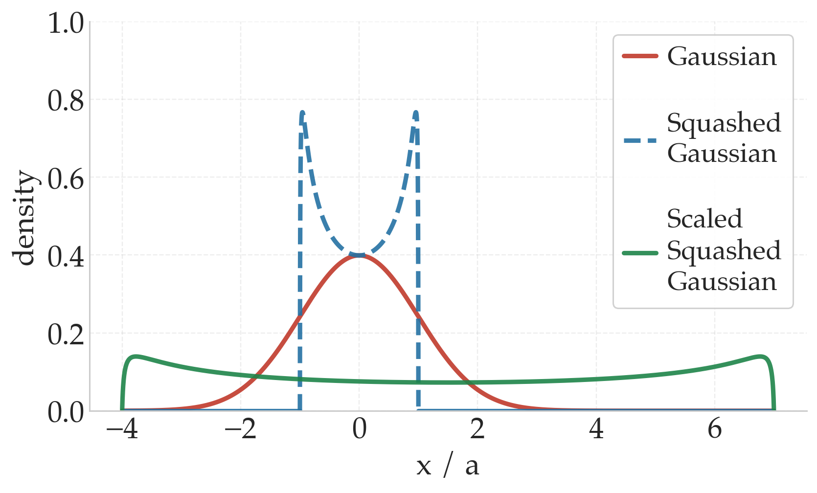
$\sigma_0 = 1.0$: near-uniform exploration
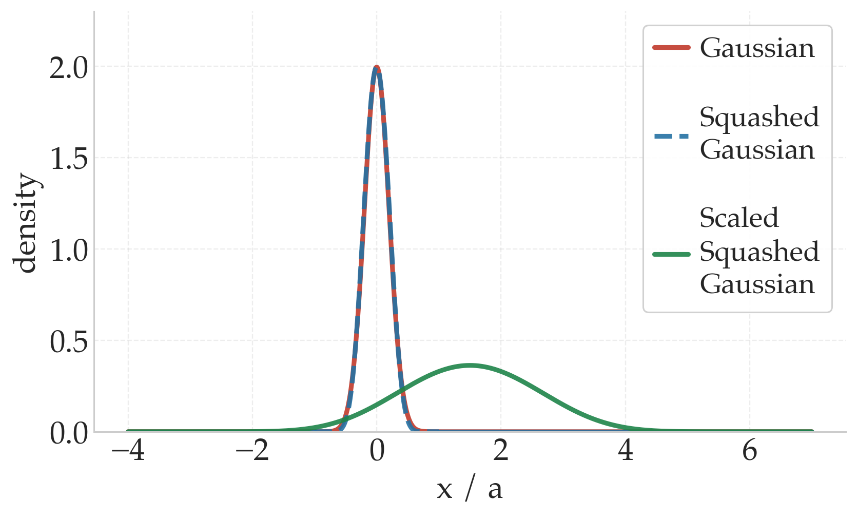
$\sigma_0 = 0.2$: concentrated exploration